Optimization
The following code demonstrates non-linear optimization by finding the best fit line to a set of points. It does not cover all the possible options or techniques available for non-linear optimization. DDogleg can solve dense and sparse systems. Unconstrained minimization and Unconstrained least-squares. Has built in support for the Schur complement. There are numerous algorithms to choose from, multiple linear solvers to select, all of which are highly configurable. See the BLAH page for a list of numerical methods available and to the BLAH techreport for a detailed discussion of the methods used internally.
Here we will tackle a problem using dense unconstrained least-squares minimization with a numerical Jacobian. Unconstrained least-squares minimization solves problems which can be described by a function of the form:
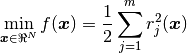
where 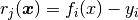 is a scalar function which outputs the residual, predicted value subtracted the observed value.
By definition
is a scalar function which outputs the residual, predicted value subtracted the observed value.
By definition  . In DDogleg you don’t define the
  function directly but instead define the set of
  functions
by implementing FunctionNtoM. Implementations of FunctionNtoM take in an array with N elements and output an array with M elements.
functions
by implementing FunctionNtoM. Implementations of FunctionNtoM take in an array with N elements and output an array with M elements.
In this example we will consider a very simple unconstrained least-squares problem, fitting a line to a set of points. To solve non-linear problems you will need to select which method to use (Levenberg Mardquardt is usually a good choise), define the function to minimize, and select an initial value. You can also specify a Jacobian, an N by M matrix which is the derivative of the residual functions. If you do not specify this function then it will be computed for you numerically.
The code below walks you through each step.
Here it is shown how to set up and perform the optimization. DDogleg is a bit unusual in that it allows you to invoke each step of the optimization manually. The advantage of that is that it is very easy to abort your optimization early if you run out of time. For sake of brevity, we use UtilProcess.optimize() to handle the iterations.
1 2 3 4 5 6 7 8 9 10 11 12 13 14 15 16 17 18 19 20 21 22 23 24 25 26 27 28 29 30 31 32 33 34 35 36 37 38 39 40 | public static void main( String args[] ) {
// define a line in 2D space as the tangent from the origin
double lineX = -2.1;
double lineY = 1.3;
// randomly generate points along the line
Random rand = new Random(234);
List<Point2D> points = new ArrayList<Point2D>();
for( int i = 0; i < 20; i++ ) {
double t = (rand.nextDouble()-0.5)*10;
points.add( new Point2D(lineX + t*lineY, lineY - t*lineX) );
}
// Define the function being optimized and create the optimizer
FunctionNtoM func = new FunctionLineDistanceEuclidean(points);
UnconstrainedLeastSquares<DMatrixRMaj> optimizer = FactoryOptimization.levenbergMarquardt(null, true);
// Send to standard out progress information
optimizer.setVerbose(System.out,0);
// if no jacobian is specified it will be computed numerically
optimizer.setFunction(func,null);
// provide it an extremely crude initial estimate of the line equation
optimizer.initialize(new double[]{-0.5,0.5},1e-12,1e-12);
// iterate 500 times or until it converges.
// Manually iteration is possible too if more control over is required
UtilOptimize.process(optimizer,500);
double found[] = optimizer.getParameters();
// see how accurately it found the solution
System.out.println("Final Error = "+optimizer.getFunctionValue());
// Compare the actual parameters to the found parameters
System.out.printf("Actual lineX %5.2f found %5.2f\n",lineX,found[0]);
System.out.printf("Actual lineY %5.2f found %5.2f\n",lineY,found[1]);
}
|
When you run this example you should see something like the following:
Steps     fx        change      |step|   f-test     g-test    tr-ratio  lambda
0     5.117E+01   0.000E+00  0.000E+00  0.000E+00  0.000E+00    0.00   1.00E-04
1     1.685E+01  -3.431E+01  1.793E+00  6.706E-01  2.279E+02   0.709   9.27E-05
2     6.133E-02  -1.679E+01  4.170E-01  9.964E-01  4.849E+01   1.026   3.09E-05
3     9.294E-06  -6.133E-02  6.479E-02  9.998E-01  3.179E-01   1.000   1.03E-05
4     2.136E-14  -9.294E-06  3.236E-04  1.000E+00  3.013E-02   1.000   3.43E-06
5     3.579E-24  -2.136E-14  3.833E-08  1.000E+00  1.929E-07   1.000   1.14E-06
6     2.792E-30  -3.579E-24  5.888E-13  1.000E+00  5.813E-12   1.000   3.81E-07
Converged g-test
Final Error = 2.791828047383737E-30
Actual lineX -2.10  found -2.10
Actual lineY  1.30  found  1.30
FunctionLineDistanceEuclidean.java
This is where the function being optimized is defined. It implements FunctionNtoM, which defines a function that takes in N inputs and generates M outputs.
Each output is the residual error for function ‘i’. Here a line in 2D is defined by a point in 2D, e.g.  .
The line passes through this point and is also tangent to the point, i.e. slope =
.
The line passes through this point and is also tangent to the point, i.e. slope =  . The error
is defined as the difference between the point and the closest point on the line.
. The error
is defined as the difference between the point and the closest point on the line.
The line is defined by two parameters so the function has two inputs. The number of outputs that it has is determined by the number of points it is being fit against. These points are specified in the constructor.
1 2 3 4 5 6 7 8 9 10 11 12 13 14 15 16 17 18 19 20 21 22 23 24 25 26 27 28 29 30 31 32 33 34 35 36 37 38 39 40 41 42 43 44 45 46 47 48 49 50 | public class FunctionLineDistanceEuclidean implements FunctionNtoM {
// Data which the line is being fit too
List<Point2D> data;
public FunctionLineDistanceEuclidean(List<Point2D> data) {
this.data = data;
}
/**
* Number of parameters used to define the line.
*/
@Override
public int getNumOfInputsN() {
return 2;
}
/**
* Number of output error functions. Two for each point.
*/
@Override
public int getNumOfOutputsM() {
return data.size()*2;
}
@Override
public void process(double[] input, double[] output) {
// tangent equation
double tanX = input[0], tanY = input[1];
// convert into parametric equation
double lineX = tanX; double lineY = tanY;
double slopeX = -tanY; double slopeY = tanX;
// compute the residual error for each point in the data set
for( int i = 0; i < data.size(); i++ ) {
Point2D p = data.get(i);
double t = slopeX * ( p.x - lineX ) + slopeY * ( p.y - lineY );
t /= slopeX * slopeX + slopeY * slopeY;
double closestX = lineX + t*slopeX;
double closestY = lineY + t*slopeY;
output[i*2] = p.x-closestX;
output[i*2+1] = p.y-closestY;
}
}
}
|